What it is
The REGBOT is DTU’s two-wheeled balancing robot — an inverted pendulum on wheels. For the final assignment in 34722 Linear Control Design 1, the job was to make it balance upright and then drive it to a commanded position, using nothing but classical frequency-domain control design. My controller is a four-loop cascade — wheel speed, balance, velocity, and position — each loop designed by hand in MATLAB, verified in Simulink against the non-linear plant, and then flashed onto the physical robot and tested on the floor.
Problem / motivation
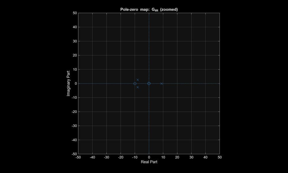
Balancing is the hard part: the plant is genuinely unstable. Linearised about upright, the balance transfer function has a right-half-plane pole at +9.13 rad/s — any tiny tilt grows like e^(9.13·t) until the robot hits the ground. It’s also non-minimum-phase (a right-half-plane zero): to accelerate forward the wheels first have to roll backward to get the centre of mass over the pivot, exactly like leaning forward before you start running. That backward-first motion is a hard physical limit on how fast the outer loops can react. A textbook PI-Lead can’t stabilise a plant like this — it needs a specific trick — and everything has to survive the jump from a clean linear model to a real robot with a real motor.
Approach
The design is a cascade: an inner wheel-speed loop, a balance loop around that, a velocity loop around that, and a position loop outermost. Each outer loop is tuned at least ~5× slower than the one inside it, so from its point of view the inner loop looks like an instantaneous unity gain.
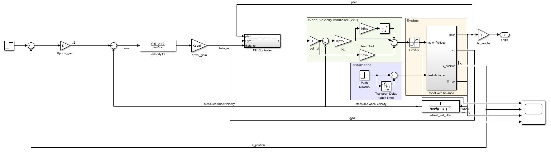
Every loop uses the same phase-balance recipe: place the PI zero from the target crossover and integrator ratio, work out how much phase lead is needed to hit a 60° phase margin at crossover, then solve the proportional gain that puts the loop gain at exactly 0 dB there. I derived each one by hand, printed every intermediate value, and checked it against MATLAB’s margin.
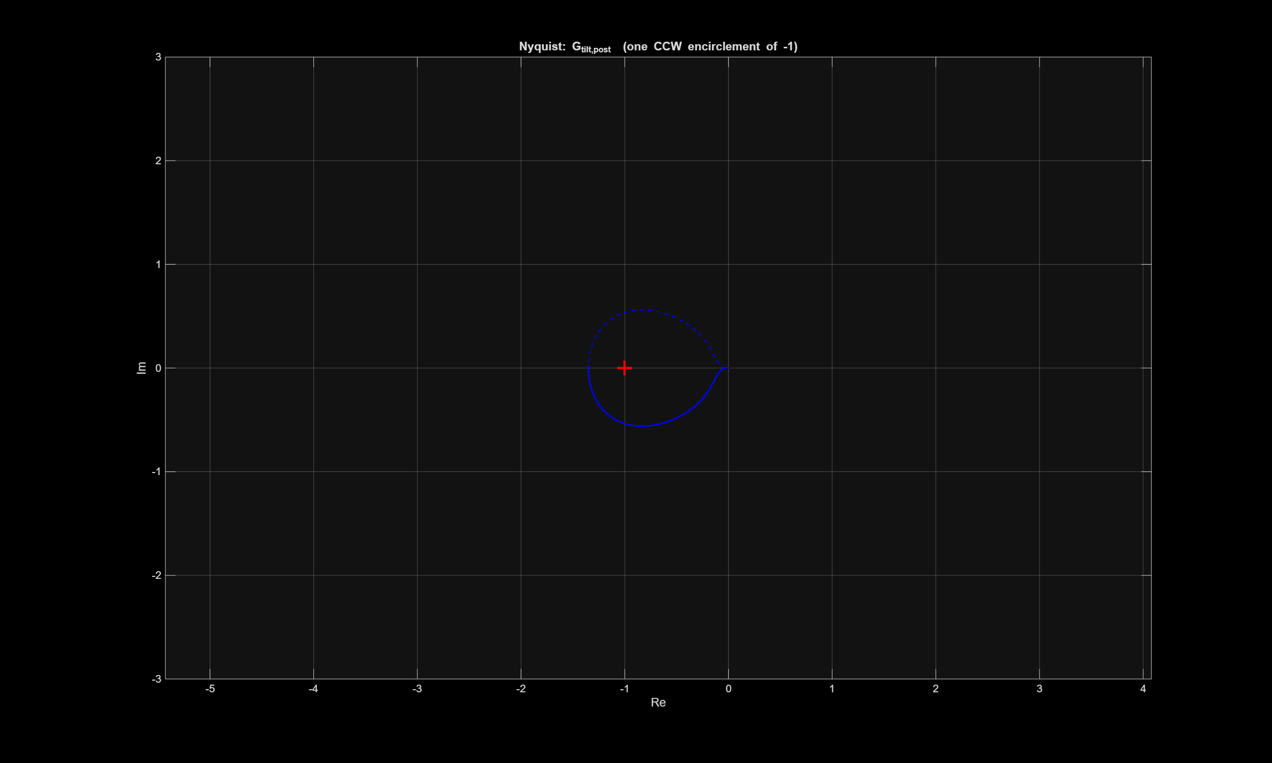
The balance loop needed more than the recipe. Because the plant is unstable, I used Lecture 10’s “Method 2”: fold a sign flip (−1) and a post-integrator — whose zero sits exactly on the plant’s magnitude peak at 8 rad/s — into the loop first. That reshapes the response so the Nyquist plot makes one counter-clockwise encirclement of −1; with one open-loop RHP pole, Z = N + P = 0, so the closed loop is stable. Only then does a normal PI-Lead go on top.
One nice shortcut: the REGBOT’s gyro measures tilt rate directly, so the derivative (Lead) term is just τ_d · gyro + θ — an ideal Lead with no noise-filter pole to design around. The whole design was validated first on the non-linear Simscape Multibody model before anything touched the hardware.
What went wrong and how it was diagnosed
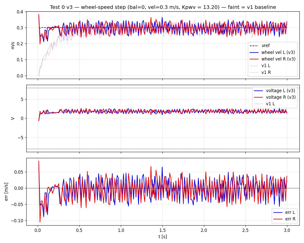
The controller met every spec on the bench and was far too slow on the floor. I first identified the motor’s voltage-to-speed plant with the robot up on blocks, wheels spinning free: G = 13.34/(s+35.71), a 28 ms time constant. Every loop designed on that model passed in simulation. Then I ran the first hardware test and the inner wheel-speed loop — designed for a 30 rad/s bandwidth — took 0.329 s to rise, the behaviour of a ~9 rad/s loop, three times slower than designed.
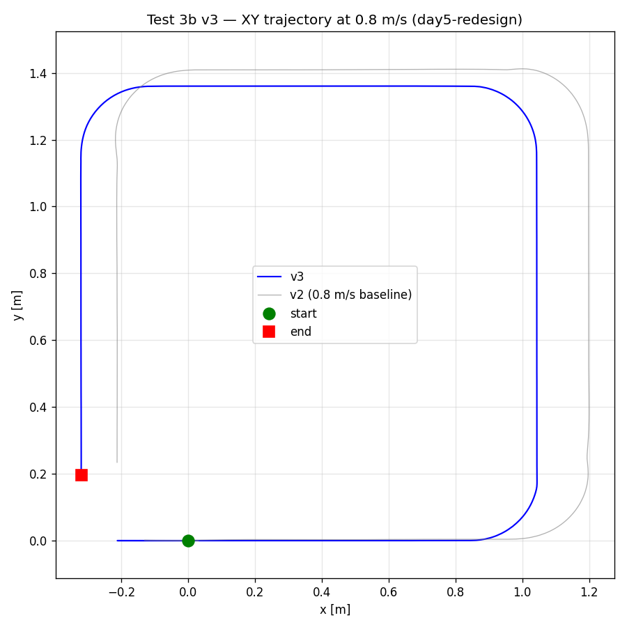
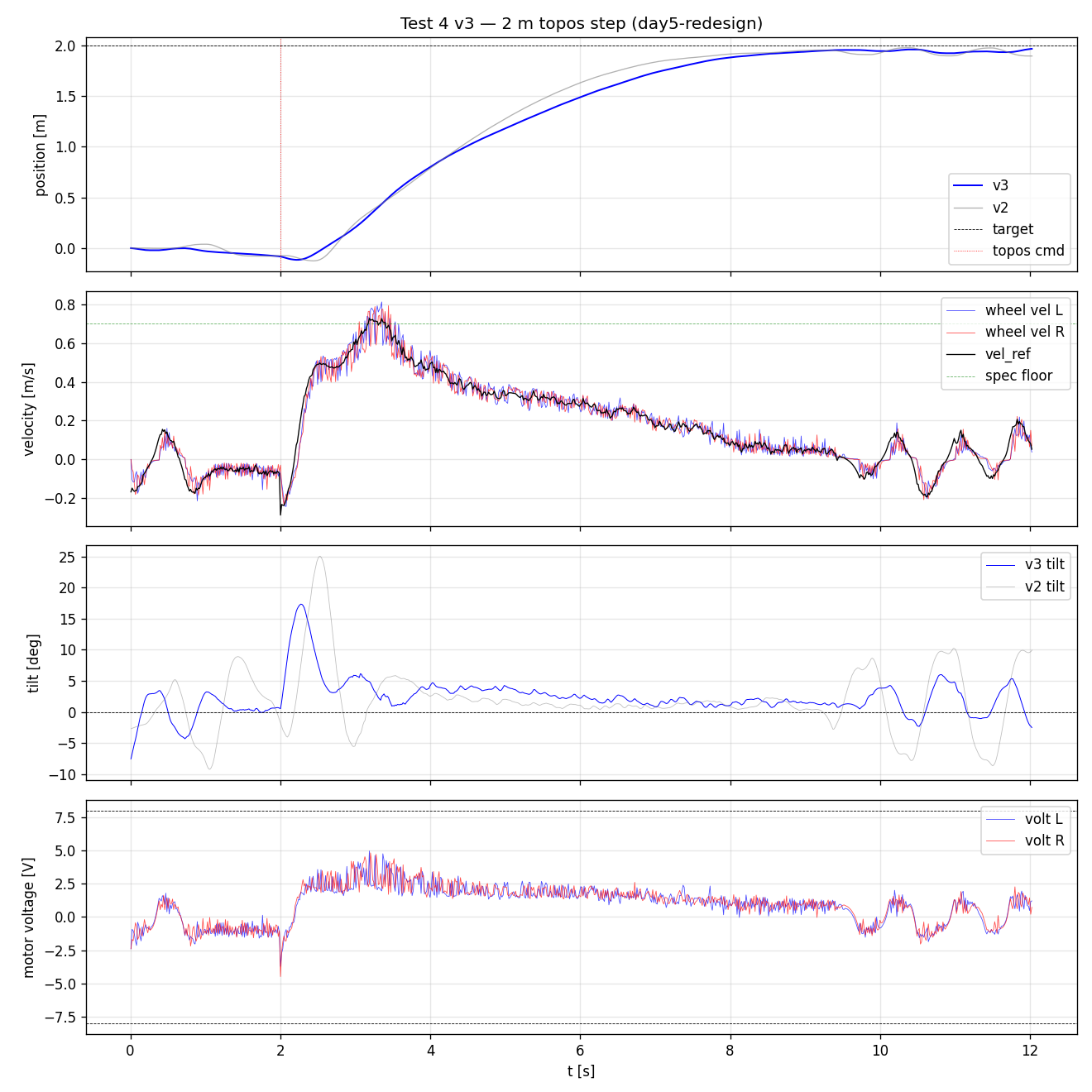
The cause was the identification itself. Wheels-up, the motor accelerates a tiny inertia and its pole sits ~6× faster than reality; on the floor it has to push the whole robot, so the real pole is much slower (G = 2.198/(s+5.985), 167 ms). I’d designed against a plant the robot never actually presents during a mission. I re-identified on the floor and re-ran all four designs — because re-linearising with the corrected inner loop shifts every outer plant too. The inner proportional gain rose 4× (3.31 → 13.20). Afterwards the same hardware test rose in 0.012 s (27× faster), the 2 m move’s final-position error improved from 10.7 cm to 3.6 cm, and a late limit cycle that had haunted the earlier runs disappeared. The honest trade-off: the inner loop now reacts ~4× harder to sharp corner commands, so peak motor voltage on the square climbed from 4.67 V to 7.31 V — 91% of the ±8 V budget.
The balance controller threw the robot over on first power-up. Method 2 hides a −1 inside the post-integrator, so the designed controller gain is effectively negative. The robot’s firmware balance block doesn’t absorb that sign itself — I’d entered the gain as a positive number, which turned the whole loop into positive feedback: the robot drove itself harder the more it tilted. The fix was one character — enter kp as −1.1999 in the firmware config — but the failure mode (a confident, accelerating fall) made the diagnosis obvious once I connected it back to the sign in the math.
Results
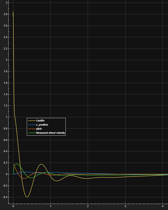
Everything was validated on the physical robot (logs recorded, plots below), all missions passing spec:
- Balance at rest, 10 s — drift 0.343 m against a 0.5 m limit.
- Square at 0.8 m/s — four sides and three turns without falling; heading returned to 359.8° (0.2° from start), peak tilt +25.5°.
- 2 m position move — final position 1.964 m (3.6 cm short), peak velocity 0.79 m/s, no overshoot and no late limit cycle.
All four loops hit their design margins (phase margins 60–83°). On the design side, the balance loop’s negative gain margin is not a bug — for an unstable plant that’s exactly what margin should report.
Tools & skills demonstrated
Classical control design end to end: system identification (tfest), frequency-domain loop shaping (PI / PI-Lead, phase-balance, Bode and Nyquist), stabilising an unstable non-minimum-phase plant with the Nyquist criterion, and cascade bandwidth budgeting. MATLAB and Simulink throughout, with a non-linear Simscape Multibody model as the verification stage between hand calculation and hardware — and the discipline to distrust a model that passed every test but disagreed with the real robot.